

GDP growth vs. household income: forward-looking scenarios for IFRS 9 expected credit losses in Kazakhstan's retail lending, 2013–2026
Authors
Yeleukenov Dauren
Share
Annotation
IFRS 9 requires forward-looking macroeconomic information in the measurement of expected credit losses (ECL); scenarios are usually built around GDP growth, and Kazakhstan's regulator recommends bounding their deviations from the consensus forecast by a corridor. Using open data for 2013–2026, the article shows that in 2016–2025 GDP growth and real household income growth were uncorrelated (correlation −0.05). The most robust driver of retail arrears is the credit cycle; household purchasing power is significant only in the full sample and only for the share of loans more than 90 days past due, and no significant negative relationship with GDP is found. The models are unstable and failed to predict the rise in arrears in 2025–2026. Scenarios built on the GDP corridor change probability-weighted ECL by less than 1%, whereas scenarios based on household income and the credit cycle increase it by 3.4–5.3%; the difference reflects mainly the narrow corridor and the unstable sign of the GDP coefficient. The article offers recommendations on choosing scenario variables for retail portfolios
Keywords
Authors
Yeleukenov Dauren
Share
IFRS 9 requires the measurement of expected credit losses (ECL) to reflect a probability-weighted amount determined over a range of possible outcomes and reasonable and supportable forecasts of economic conditions (IFRS Foundation, 2014), and the Basel Committee on Banking Supervision (BCBS, 2015) regards the supportability of such information as a key element of provisioning. In practice, the requirement is implemented through a satellite model and a set of macroeconomic scenarios whose assumptions differ considerably across banks (European Banking Authority, 2023).
In Kazakhstan, the regulator has intervened in scenario selection directly. In 2022, citing bank disclosures with economic growth forecasts of up to 10%, the Agency of the Republic of Kazakhstan for Regulation and Development of Financial Market (ARDFM) published a consensus forecast with permissible deviations of no more than 1.6 percentage points (pp) above and 2.3 pp below for GDP growth and 0.6–1.2 pp for inflation; banks are advised to assign at least half of the weight to the consensus, and material unjustified deviations are subject to additional supervisory checks (ARDFM, 2022). The baseline scenario of the supervisory stress test is also built on a consensus of forecasts by government agencies and international organizations (ARDFM, 2024).
GDP is the anchor variable of this framework. Yet in 2025, real GDP grew by 6.5% on average, real household money income (hereafter, real income) fell by 0.6%, and the share of retail loans more than 90 days past due (90+ dpd) rose from 3.82% at the end of 2024 to 4.80% on July 1, 2026 (ARDFM, 2012–2026; Bureau of National Statistics [BNS], n.d.). The official forecast offers alternative variants only for economic growth (Government of the Republic of Kazakhstan, 2025). Retail loans account for 57.8% of the banks’ loan portfolio (ARDFM, 2012–2026).
The literature confirms that GDP growth is a leading driver of non-performing loans (Beck et al., 2015; Louzis et al., 2012), but the evidence for Kazakhstan is mixed: significant drivers include the output gap, the credit-to-GDP gap, and asset prices (Podlich et al., 2010); the coefficient on GDP growth is positive in annual data (Zaitenova & Baibulekova, 2016); and household debt burden responds most strongly to income shocks (Aldashev & Batkeyev, 2023). The National Bank of Kazakhstan (NBK, 2018, 2026) links macroeconomic scenarios to IFRS 9 stages using credit registry data. To the author’s knowledge, no study has used open data to test the choice of scenario variables for retail lending in Kazakhstan.
Objective
This study uses open data for 2013–2026 to test whether GDP growth explains the dynamics of retail loan arrears at Kazakhstan’s banks better than real income and the credit cycle, and to assess how the choice of scenario variables affects probability-weighted ECL when the regulator’s recommendations on the deviation corridor and on the weight of the consensus forecast are followed.
Materials and Methods
Data. Loan quality indicators (principal outstanding, including retail loans) were taken from 59 quarterly (beginning-of-quarter) issues of the ARDFM bulletin Current State of the Banking Sector of the Republic of Kazakhstan for 2012–2026 (ARDFM, 2012–2026); the retail 90+ dpd series covers 2013Q2–2026Q2. GDP, real income, and consumer price indices were obtained from the BNS (n.d.).
Dependent variable. The dependent variable is the annual change in the logit of the retail 90+ dpd share:
ΔL₄,ₜ = logit(NPLₜ) − logit(NPLₜ₋₄), logit(p) = ln(p / (100 − p)),
where NPLₜ is the share of retail loans 90+ dpd at the end of quarter t, %. Most of the decline in this share (from 18.99% in 2013Q2 to 3.82% in 2024Q4) occurred in quarters with one-off write-offs and transfers of problem assets (for the 2014–2017 episodes, see NBK, 2018), and quarterly changes are not explained by macroeconomic variables (adjusted R² of −0.025). The analysis therefore uses an annual horizon, which coincides with the 12-month ECL horizon for Stage 1.
Models. The estimated regression is
ΔL₄,ₜ = α + β · Xₜ + γ₀ · CRₜ + γ₄ · CRₜ₋₄ + εₜ,
where Xₜ is annual growth in real GDP or real income, %, and CRₜ is annual growth in the retail loan portfolio, %; γ₀ captures the denominator effect, and γ₄ the seasoning of loans issued during a credit boom. Models M1 (GDP), M2 (income), and M3 (GDP and income) include CRₜ₋₄; M4 (income), M5 (GDP), and M8 (inflation) include both CRₜ and CRₜ₋₄; M6 and M7 add inflation to M4 and M5, respectively. The main sample is 2016Q1–2026Q2 (after the move to a floating exchange rate); standard errors are Newey–West with four lags (Newey & West, 1987).
Robustness checks. The models are estimated on subsamples, over a 24-quarter rolling window, and out of sample (estimation through 2024Q4, forecast for 2025–2026H1). The dependent variable is also replaced with a measure of arrears inflow: the share of loans 61–90 dpd, which is not yet affected by write-offs (four-quarter moving average). A structural break in 2022Q1 is tested with a Wald test.
Mapping to ECL. The scenario shift in the logit of the 12-month probability of default (PD) equals Σ βₖ · ΔXₖ, where ΔXₖ is the deviation of variable k from the baseline scenario (an assumption made for illustration). ECL for a stylized unsecured retail segment equal PD × LGD × EAD, where LGD is loss given default and EAD is exposure at default; EAD is KZT 100 billion, LGD is 75%, and the baseline PD is 5.0%.
Results
1. Divergence Between GDP Growth and Real Income
In 2016–2025, the correlation between annual growth rates of real GDP and real income was −0.05 (Figure 1), and the coefficient from a regression of income growth on GDP growth was insignificant (t = −0.27). In 2022Q4–2023Q1 and 2025Q2–Q4, GDP grew by more than 3% while real income declined; both episodes coincided with accelerating inflation and a credit boom. A lower GDP path in a downside scenario therefore does not necessarily pass through to retail borrowers.
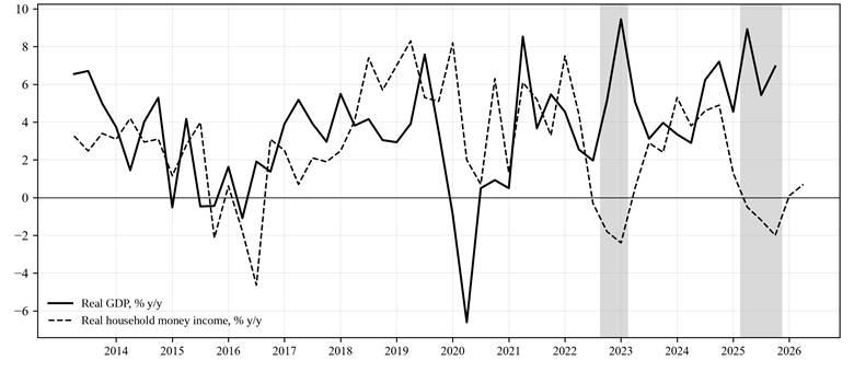
Figure 1. Growth in real GDP and real household money income in Kazakhstan, % change from the same quarter of the previous year. Shaded areas mark quarters in which GDP grew by more than 3% while real income declined. Source: compiled by the author from BNS (n.d.) data.
2. Models of the Annual Change in Retail Arrears
Table 1. Annual change in the logit of the retail 90+ dpd share, 2016Q1–2026Q2 (coefficient, t-statistic in parentheses)
|
Variable |
M1 |
M2 |
M3 |
M4 |
M5 |
|
Real GDP growth, % |
0.0088 (0.97) |
– |
0.0081 (1.22) |
– |
0.0166 (2.49) |
|
Real income growth, % |
– |
−0.0250 (−4.00) |
−0.0231 (−3.90) |
−0.0180 (−2.49) |
– |
|
Retail portfolio growth, % |
– |
– |
– |
−0.0059 (−1.60) |
−0.0105 (−4.06) |
|
Retail portfolio growth 4 quarters earlier, % |
0.0062 (2.86) |
0.0060 (3.21) |
0.0055 (3.13) |
0.0096 (3.05) |
0.0118 (4.80) |
|
Observations |
40 |
42 |
40 |
42 |
40 |
|
Adjusted R² |
0.18 |
0.39 |
0.38 |
0.44 |
0.41 |
Source: author’s calculations. Newey–West standard errors, four lags. Models with GDP have fewer observations because quarterly GDP data for 2026 have not yet been published.
The real-income model (M2) explains twice as much of the variation as the GDP model (M1): adjusted R² of 0.39 versus 0.18 with 42 and 40 observations, respectively (Table 1). The income coefficient is negative and significant, whereas the GDP coefficient is insignificant, including in M3. Portfolio growth a year earlier raises arrears (seasoning), while current growth reduces their share (the denominator effect). With the credit cycle included (M5), the GDP coefficient is significant but positive: faster economic growth was accompanied by rising, not falling, retail arrears.
3. Robustness
Across subsamples (2016–2021, 2016–2024, and 2019–2026), the coefficients on the macroeconomic variables are unstable: the income coefficient (M4) is not significant at the 5% level in any of them, and the GDP coefficient (M5) is negative in 2016–2021 (−0.0094, t = −1.82) but positive in the samples that include 2022–2026; in the rolling window, the GDP coefficient changes sign once and the income coefficient four times. The sign of the denominator effect is stable: the coefficient on current portfolio growth is negative in all subsamples (insignificant in 2019–2026), and the seasoning effect appears from 2019 onward. The Wald test rejects coefficient stability across the 2022Q1 break at the 1% level (F = 20.23 for M4 and 23.67 for M5).
The decline in real income coincided with accelerating inflation: when inflation is added (M6), the income coefficient loses significance (−0.0103, t = −0.95), and the model with inflation instead of income (M8) explains the same share of the variation (adjusted R² 0.44; inflation coefficient 0.0132, t = 2.10), so in aggregate data both indicators capture household purchasing power. The GDP coefficient remains positive and significant when inflation is included (M7: 0.0152, t = 2.27).
All four models (M1, M2, M4, and M5) estimated on data through end-2024 predicted a decline in the logit of retail arrears in 2025–2026H1 (−0.061 to −0.119 per year), whereas it actually rose by 0.127 per year; that is, the odds of arrears increased by about 13.5% annually. The income models had smaller errors (root mean square error of 0.189–0.194 versus 0.210–0.246), but none captured the direction of change. This conclusion does not depend on the increase in the number of banks in 2025Q2–Q3 (ARDFM, 2012–2026): the forecasts diverged from actual values as early as 2025Q1–Q2, and the arrears inflow had already risen in 2024.
Arrears inflow. For the 61–90 dpd share, the credit cycle effect is stronger (both coefficients significant, |t| > 5; adjusted R² up to 0.72), the GDP coefficient is positive and significant in all subsamples (0.0352, t = 3.66 in the full sample), and real income and inflation are insignificant in the full sample. The link with purchasing power is thus confirmed only for the 90+ dpd share; a possible explanation is that falling income makes it harder to exit arrears but does not determine entry into them. The arrears inflow rose in 2024 (from 0.46% to 0.58%), a year before the 90+ dpd share increased.
4. Implications for ECL Scenarios
Two scenario sets are compared. Set A follows the ARDFM corridor: GDP growth is 2.3 pp below the consensus in the downside scenario and 1.6 pp above it in the upside scenario, with PD mapping by model M5. Set B uses variables linked to retail arrears: in the downside scenario, real income falls by 4.6% (the series minimum) against 2.0% growth in the baseline, and portfolio growth slows to 2% against 14%; in the upside scenario, income grows by 4.0% and the portfolio by 18%; PD mapping uses model M4. The baseline values are the author’s assumptions, because income forecasts are not published in variants (Government of the Republic of Kazakhstan, 2025).
In Set A, the downside scenario lowers ECL by 3.6% and the upside scenario raises it by 2.6%: the empirical sign is the opposite of the one presumed by the corridor design. In Set B (with full-sample coefficients), the downside scenario raises PD from 5.00% to 5.98% and ECL by 19.6%, while the upside scenario lowers ECL by 5.5%. More than half of the logit shift comes from the income coefficient, which is unstable across subsamples (Section 3); the contribution of slower lending reflects a change in the portfolio’s age composition rather than a deterioration in borrowers’ ability to pay.
Even with a “classical” negative, albeit insignificant, GDP coefficient (2016–2021 subsample, t = −1.82), a deviation at the corridor boundary increases ECL by only 2.1% (and lowers it by 1.4% on the upside). A shock as severe as in Set B, namely a 6.6% fall in GDP as in 2020Q2, or 12.0 pp below the baseline (5.4%), increases ECL by 11.3% under the “classical” sign and reduces it by 17.3% under the estimated sign. Because the corridor is narrow, a GDP scenario changes ECL little, and because the sign is unstable, the direction of the change is unpredictable.
Table 2 reports probability-weighted ECL under weights consistent with the recommendation to assign at least half of the weight to the consensus forecast.
Table 2. Probability-weighted 12-month ECL, KZT billion (change from the baseline scenario, %, in parentheses)
|
Weights: baseline / downside / upside |
Set A (GDP corridor, estimated sign) |
Set A (GDP corridor, “classical” sign) |
Set B (income and credit cycle) |
|
50 / 25 / 25 |
3.741 (−0.3) |
3.756 (+0.2) |
3.882 (+3.5) |
|
60 / 30 / 10 |
3.719 (−0.8) |
3.768 (+0.5) |
3.950 (+5.3) |
|
70 / 20 / 10 |
3.733 (−0.5) |
3.760 (+0.3) |
3.877 (+3.4) |
Source: author’s calculations.
Under Set A, weighting does not increase the allowance, and under the “classical” sign it raises it by only 0.2–0.5%: the procedure is formally complied with, but the uncertainty of retail credit risk does not enter the estimate. Under Set B, weighted ECL are 3.4–5.3% above the baseline.
The inflation corridor (1.2 pp) is 11 times narrower than the largest annual change in inflation in 2016–2026 (13.4 pp): under M8, a deviation at its boundary raises PD only to 5.08%, versus 5.91% under the historical shock.
Discussion and Recommendations
These results do not imply that a deep general downturn would leave borrowers unaffected: the sample contains only one such episode, in 2020, which was cushioned by payment deferrals. However, in 2016–2026, GDP growth was not a sufficient variable for constructing retail scenarios. In the author’s view, the reasons are the large share of the commodity sector in GDP growth, the weak pass-through of this growth to household income, and the coincidence of faster growth with credit booms and inflation.
The results lead to the following recommendations for banks and the regulator:
- Build retail scenarios primarily on credit cycle indicators, supplemented by real income and inflation.
- Add real household income to the regulator’s consensus forecast and set the corridor bounds with reference to historical annual changes in the indicators.
- Test the sign and stability of satellite model coefficients out of sample: a model with a sign opposite to the expected one turns the downside scenario into a factor that reduces the allowance.
- Where models are unstable, apply post-model adjustments with explicit triggers (an accelerating arrears inflow, divergence between GDP and real income growth).
Limitations of the study: aggregate data (42 overlapping annual changes) reduce statistical power and do not allow effects to be separated by bank and product; the 90+ dpd share depends on write-offs; and the parameters of the stylized segment are set by the author. A more precise test is possible using credit registry data (NBK, 2026).
References:
- In 2016–2025, real GDP growth and real income growth in Kazakhstan were virtually unrelated (correlation −0.05).
- The most robust driver of retail arrears is the credit cycle; household purchasing power is significant only in the full sample and only for the 90+ dpd share, and no significant negative relationship with GDP was found.
- Aggregate satellite models are unstable and failed to predict the rise in retail arrears in 2025–2026, even though the arrears inflow had risen a year earlier.
- Scenarios based on the GDP corridor change probability-weighted ECL by less than 1%, whereas scenarios based on income and the credit cycle (with full-sample coefficients) increase them by 3.4–5.3%; the difference stems mainly from the narrowness of the corridor and the instability of the sign of the GDP coefficient.
References
Agency of the Republic of Kazakhstan for Regulation and Development of Financial Market. (2012–2026). Current state of the banking sector of the Republic of Kazakhstan (Monthly issues, January 1, 2012–July 1, 2026) [In Russian]. https://www.gov.kz/memleket/entities/ardfm/press/article/details/72350?lang=ru
Agency of the Republic of Kazakhstan for Regulation and Development of Financial Market. (2022). Review of macroeconomic forecasts: Consensus forecast, decomposition, range of potential values [In Russian]. https://www.gov.kz/uploads/2022/1/25/8d1785206ad5c917189346450b520c1f_original.960419.pdf
Agency of the Republic of Kazakhstan for Regulation and Development of Financial Market. (2024). Report on the 2023 supervisory stress testing of banks [In Russian]. https://www.gov.kz/uploads/2024/5/22/9096746064a9139153adb62ad19bbc7b_original.1707429.pdf
Aldashev, A., & Batkeyev, B. (2023). Household debt, heterogeneity and financial stability: Evidence from Kazakhstan. Central Bank Review, 23(2), Article 100119. https://doi.org/10.1016/j.cbrev.2023.100119
Basel Committee on Banking Supervision. (2015). Guidance on credit risk and accounting for expected credit losses. Bank for International Settlements. https://www.bis.org/bcbs/publ/d350.pdf
Beck, R., Jakubík, P., & Piloiu, A. (2015). Key determinants of non-performing loans: New evidence from a global sample. Open Economies Review, 26(3), 525–550. https://doi.org/10.1007/s11079-015-9358-8
Bureau of National Statistics of the Agency for Strategic Planning and Reforms of the Republic of Kazakhstan. (n.d.). GDP by the production method (quarterly); Index of real money income; Consumer price index by 13 main divisions [Data set, in Russian]. https://stat.gov.kz/ru/industries/economy/national-accounts/dynamic-tables/
European Banking Authority. (2023). IFRS 9 implementation by EU institutions: 2023 monitoring report (EBA/Rep/2023/36). https://www.eba.europa.eu/sites/default/files/2023-11/25b12d35-9c28-4335-a589-166c77198920/Final%20Report%20on%20IFRS9%20implementation%20by%20EU%20institutions.pdf
Government of the Republic of Kazakhstan. (2025). Forecast of the socio-economic development of the Republic of Kazakhstan for 2026–2028 (Approved at the Government meeting of August 26, 2025, Minutes No. 32) [In Russian]. https://www.gov.kz/uploads/2025/9/17/f2e7461f559e6c02ad52a135d89c7d3c_original.647617.pdf
IFRS Foundation. (2014). IFRS 9 Financial Instruments (as amended).
Louzis, D. P., Vouldis, A. T., & Metaxas, V. L. (2012). Macroeconomic and bank-specific determinants of non-performing loans in Greece: A comparative study of mortgage, business and consumer loan portfolios. Journal of Banking & Finance, 36(4), 1012–1027. https://doi.org/10.1016/j.jbankfin.2011.10.012
National Bank of Kazakhstan. (2018). Financial stability report of Kazakhstan 2015–2017. https://nationalbank.kz/file/download/40526
National Bank of Kazakhstan. (2026). Financial stability report of Kazakhstan 2025. https://nationalbank.kz/file/download/137846
Newey, W. K., & West, K. D. (1987). A simple, positive semi-definite, heteroskedasticity and autocorrelation consistent covariance matrix. Econometrica, 55(3), 703–708. https://doi.org/10.2307/1913610
Podlich, N., Illyasov, D., Tsoy, E., & Shaikh, S. (2010). The methodology of stress tests for the Kazakh banking system (Ifo Working Paper No. 85). Ifo Institute.
Zaitenova, N., & Baibulekova, L. (2016). Evaluation of influence of macroeconomic shocks on the banking sector of Kazakhstan. International Journal of Economics and Financial Issues, 6(S2), 188–194.
Other articles of the issue